
Product / Simulate
Every result ships with the setup and evidence that produced it.
Fixtures, loads, materials, interface policies, mesh settings, and solved fields stay attached to the design. Every result reports the mesh it was actually solved on, its force balance, a plausibility check, and the solver build that produced it.
Simulate workspace
Results are part of the document, not a screenshot.
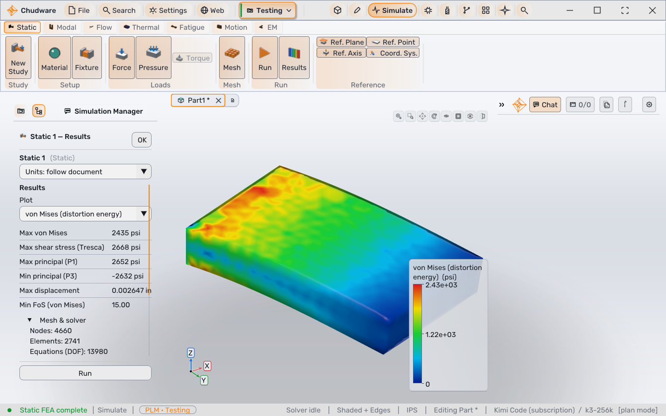
A solved study can display stress, displacement, factor of safety, temperature, mode shape, or the field appropriate to that analysis. The results panel keeps scalar summaries and mesh information beside the viewport instead of separating the color plot from its setup.
Study types
Choose the analysis that matches the question.
Each study uses the real part or assembly mesh. The solver's scope and assumptions differ by study and remain part of the result.
| Static stress | Linear-elastic tet10 solve by default, with forces or pressures, picked fixtures, per-body materials, optional bonded interfaces, and factor-of-safety fields. |
|---|---|
| Adaptive and convergence | Error-driven remesh-and-resolve passes, or an explicit coarse-to-fine size ladder with the monitored result and delta reported per leg. |
| Contact | Frictionless unilateral contact for separated bodies, with bonded, contact, and free pair policies, local interface refinement, active-set convergence, and contact diagnostics. |
| Modal and frequency response | Natural frequencies and mode shapes, followed by harmonic response through modal superposition with the supplied damping assumption. |
| Thermal | Steady or transient conduction with fixed temperatures, heat flux, convection, and scheduled transient loads. |
| Buckling | Linear eigenvalue buckling modes and load factors for a stated reference load. |
| Fatigue | High-cycle S-N evaluation from the static stress field with selectable mean-stress theory and endurance corrections. |
| Flow | Built-in voxel flow for directional comparisons, plus an OpenFOAM external-aerodynamics path when OpenFOAM is installed. |
Study setup
Boundary conditions and mesh are explicit, never guessed.
Select the study and material model
Use a named material or explicit properties. Multi-body static and contact studies can assign a different material to each body.
Resolve fixtures, loads, and thermal boundaries to faces
Picked faces and stable face identifiers tie the setup to document geometry. Preview the selections before solving.
Declare assembly interfaces
Classify relevant body pairs as bonded, contact, or free. A contact study can mix bonded and unilateral-contact pairs in the same assembly.
Choose and inspect the mesh
Set an explicit characteristic size when the discretization must be reproducible. Contact studies can refine only the interface; convergence studies solve a declared size ladder.
Evidence returned with a solve
Check more than the peak value.
Static and adaptive results return mesh quality, applied and reaction resultants, equilibrium error, and a displacement-to-part-size plausibility check beside the stress summary. A mechanism or disconnected unfixed body is refused rather than presented as a small stress.
Result provenance includes the engine build, pinned PolyMesh commit, solver, mesher, and timestamp. Optional VTU output carries the solved fields for independent inspection in ParaView or another compatible tool.
A convergence run records requested and delivered element size, nodes, elements, degrees of freedom, the monitored quantity, and the change from the previous leg. Identical or implausible legs do not count as convergence.
| Setup | Material, fixtures, loads, body roster, and interface policy |
|---|---|
| Delivered mesh | Element order, characteristic size, node and element counts, aspect and Jacobian metrics, poor-element percentage, connected components |
| Balance | Applied and reaction force and moment, with equilibrium error |
| Plausibility | Maximum displacement compared with the part's bounding-box diagonal |
| Stress reduction | Reported peak plus the raw value and the mask used to exclude the fixture-ring singularity from selected summaries |
| Provenance | Engine build, PolyMesh commit, solver, mesher, and timestamp |
Mesh sensitivity
Prove the mesh before you trust the number.
One fine-looking mesh doesn't prove the number you're about to act on is stable. Run the same setup at several element sizes and compare the result across the meshes that were actually delivered.
Adaptive refinement targets high estimated discretization error. The estimator is an indicator, not a bound on physical error; singularities, boundary-condition assumptions, and material-model limits still require engineering judgment.
Model boundaries
Know what each solver does not represent.
The default static path is small-displacement, isotropic linear elasticity. Optional small-strain J2 plasticity can redistribute load when explicitly enabled, but it is not a large-deformation or general nonlinear material solver.
Contact is frictionless and pairs surfaces on the undeformed mesh. It models opening and compressive transfer, not large sliding, friction, or bolt preload. Linear buckling predicts eigenvalue load factors, not post-buckling collapse.
The built-in voxel-flow result is for directional comparison. Use the separately installed OpenFOAM path for higher-fidelity external-aerodynamics work, and still perform mesh and convergence review.
Engineering responsibility
Simulation is evidence for a decision, not certification of a design. Check the geometry, boundary conditions, material data, units, mesh resolution, balance, convergence, and solver assumptions against the physical problem.
A result that violates its model assumptions is diagnostic output, even when the solver converged.
Next
Run a study on your own part.
Start with a representative load case, then inspect the mesh and evidence before refining the result.